Goalie-Specific Priors on Save Probability
In a previous post, I motivated and created a theoretical win probability model. I explored a few different ways to choose parameters that the model depends on, but one way that I haven’t written about (but have started using) is using goalie-specific priors. In all of the previous models, I assumed the same prior on all goalies for ease of computation. In practice, however, we know that some goalies are better than others (Connor Hellebuyck, Igor Shesterkin, and Andrei Vasilevskiy come to mind), while others are much worse. Therefore, it may improve the prediction accuracy of the model if we estimate priors specifically for each goalie using exclusively their starts, and at the very least, it should result in win probability estimates and goalie recommendations that make more intuitive sense.
To choose the parameters for a specific game, I’m going to consider all regular-season games within the past calendar year as the prior data. This should give us a large enough sample to obtain appropriate estimates, while also ensuring that we’re not using irrelevant data. For the distributions on shots on goal per game, I’m again going to train a negative binomial distribution on this prior data set, using the team and a binary home/away variable to get parameter estimates. For the priors on save probability, there are two potential options. If the goalie has played at least 10 games in the past calendar year, I’ll simply use all of that goalie’s starts and use maximum-likelihood estimations to obtain the best estimates for \(\alpha\) and \(\beta\) for that particular goalie’s Beta distribution on save probability. If the goalie has played fewer than 10 games in the past calendar year, I’ll use all starting performances from that goalie’s team to get a prior. This isn’t perfect – ideally I’d like to use a “replacement-level prior” for goalies with insufficient starts, but that’s not the easiest thing to compute, so the next-best thing is to just assume that a goalie with insufficient information will simply be a plug-in goalie for whichever team he’s playing for.
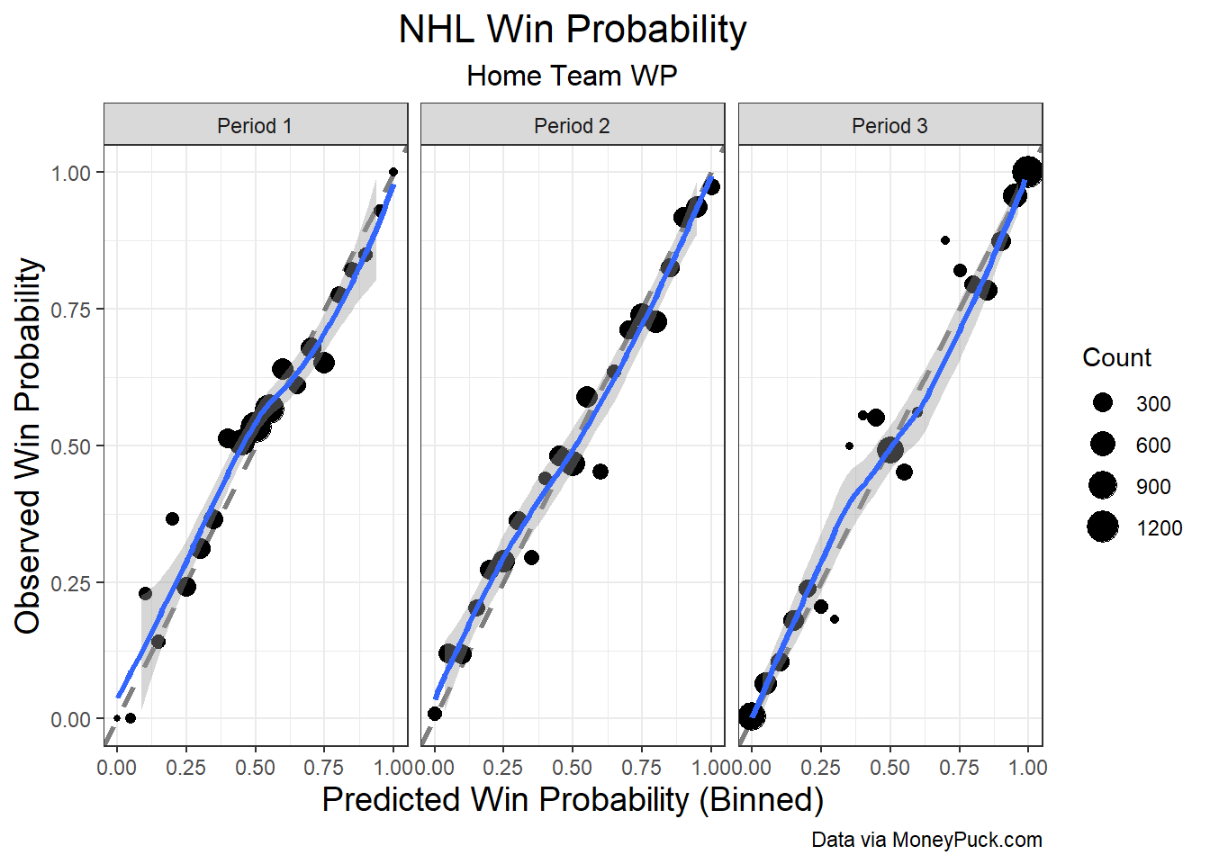
To control the evaluation as best as possible, I’m going to use the same methodology as in the original post and the same list of sampled evaluation points. For this updated model, the binned vs. observed win probability graphs are shown below:

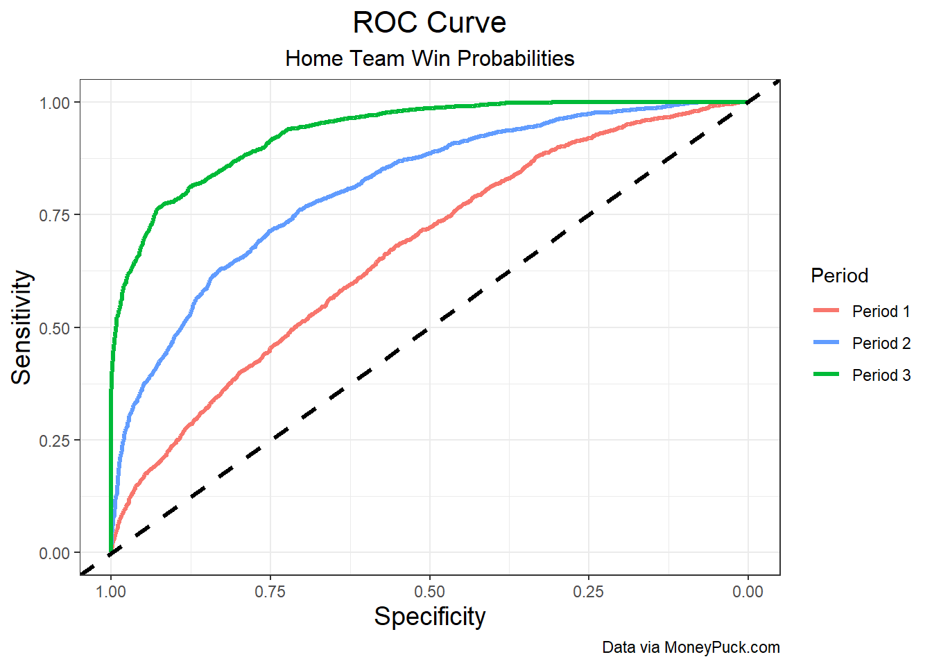
This model looks good, although it suffers from some of the same drawbacks as the best model from the original post. Nevertheless, the model is definitely not any worse, so I’ll be using this model going forward, as the numbers we get as output make more intuitive sense to a regular observer. The ROC curves for this model are shown below.

This model gives a log-loss of 0.644 for the first period, 0.529 for the second period, and 0.317 for the third period. The AUC for the three ROC curves are 0.667 for the first period, 0.81 for the second period, and 0.934 for the third period. Comparing these results with those from the original post, we see some marginal improvement by using this model, which further justifies the use of this particular model going forward.